Implementing Stochastic Gradient Descent and variants from scratch.
In this post, we implemented stochastic gradient descent in python which is one of the efficient method for training ML models. The implementation encompases various SGD variants like constant and shrinking step sizes, momentum, and averaging, comparing how each one impacts the speed and accuracy of the model's convergence.
Welcome to the implementation of an important optimization techniques in machine learning! In this post, we’ll look at Gradient Descent (GD) and Stochastic Gradient Descent (SGD) which are two essential methods for training machine learning models. Whether you’re new to these concepts or looking to refine your understanding, this post is designed to make these methods comprehensive and practical.
We’ll walk through various SGD variants like constant and shrinking step sizes, momentum, and averaging, comparing how each one impacts the speed and accuracy of the model’s convergence. Along the way, we’ll discuss when to use each technique, what makes them effective, and how to balance computational cost with performance.
Let’s dive in together and discover the best method for training your machine learning model!
1
2
3
4
5
6
7
# The following libraries will be essential for our implemetation.
import numpy as np
from numpy import linalg as la
from scipy.linalg import norm
import matplotlib.pyplot as plt
from numba import njit, jit  # A just in time compiler to speed things up!
%matplotlib inline
Linear Regression with Ridge Penalization
In our linear regression model with Ridge penalization, the goal is to find the weight vector \(w\) that minimizes the following objective function:
\begin{equation} \label{eq:linear-regression} f(w) = \frac{1}{2n} |Xw - y|^2 + \frac{\lambda}{2} ||w||^2, \end{equation}
where \(X\) is our feature matrix, \(y\) is the vector of true values, and \(\lambda\) is the regularization parameter that controls the strength of the penalty on the size of the weights.
To optimize this objective function using gradient-based methods, we need to compute the gradient, which tells us the direction in which the function decreases most rapidly. The gradient of the objective function \(f(w)\)is:
\begin{equation} \label{eq:gradient} \nabla f(w) = \frac{1}{n} X^T(Xw - y) + \lambda w, \end{equation}
where the first term \(\frac{1}{n} X^T(Xw - y)\) represents the gradient of the least-squares loss, while the second term \(\lambda w\) accounts for the regularization.
For stochastic gradient descent (SGD), we often update the weights using the gradient calculated from a single data point rather than the entire dataset. The gradient for a single data point \(i\) is given by:
\begin{equation} \label{eq:sgd} \nabla f_i(w) = (X_i w - y_i) X_i + \lambda w \end{equation}
We will implement this as well which will allow us to perform efficient updates in each iteration of SGD.”
To ensure stable and efficient updates in gradient-based methods, it’s important to set an appropriate step size. The Lipschitz constant \(L\) provides an upper bound on the gradient’s rate of change and helps in choosing this step size:
\begin{equation} \label{eq:step-size} L = \frac{|X|_2^2}{n} + \lambda, \end{equation}
which guides us in selecting a step size that prevents overshooting during optimization.
In stochastic gradient descent, where updates are made based on individual data points, the step size can be adapted to the specific characteristics of each data point.
\begin{equation} \label{eq:lmax} L_{\text{max}} = \max\left(\sum X_i^2\right) + \lambda \end{equation}
This constant ensures that the step size is appropriately scaled, even for the most ‘difficult’ data points, preventing instability in the updates.
Lastly, when dealing with strongly convex functions, the strong convexity constant \(\mu\) provides a lower bound on the curvature of the objective function.
\begin{equation} \label{eq:muconstant} \mu = \frac{\min(\text{eigenvalues}(X^TX))}{n} + \lambda \end{equation}
The strong convexity constant helps in determining how aggressively we can update our weights without risking divergence.
Lets now put all the pieces we’ve discussed above into a LinReg class which will be important for our optimization tasks.
1
2
3
4
5
6
7
8
9
10
11
12
13
14
15
16
17
18
19
20
21
22
23
24
25
26
27
28
29
30
31
32
from scipy.linalg import svd

class LinearRegression(object):
    def __init__(self, X, y, lbda):
        self.X = X
        self.y = y
        self.n, self.d = X.shape
        self.lbda = lbda
    def grad(self, w):
        return self.X.T.dot(self.X.dot(w) - self.y) / self.n + self.lbda * w

    def f_i(self, i, w):
        return norm(self.X[i].dot(w) - self.y[i]) ** 2 / (2.) + self.lbda * norm(w) ** 2 / 2.

    def f(self, w):
        return norm(self.X.dot(w) - self.y) ** 2 / (2. * self.n) + self.lbda * norm(w) ** 2 / 2.

    def grad_i(self, i, w):
        x_i = self.X[i]
        return (x_i.dot(w) - self.y[i]) * x_i + self.lbda * w

    def lipschitz_constant(self):
        L = norm(self.X, ord=2) ** 2 / self.n + self.lbda
        return L

    def L_max_constant(self):
        L_max = np.max(np.sum(self.X ** 2, axis=1)) + self.lbda
        return L_max

    def mu_constant(self):
        mu =  min(abs(la.eigvals(np.dot(self.X.T,self.X)))) / self.n + self.lbda
        return mu
Whether you’re using full-batch gradient descent or stochastic methods, this class forms the backbone of our optimization experiments, enabling us to test and compare different techniques effectively.
Logistic Regression with Ridge Penalization
Similarly, in logistic regression, our goal is to find the weight vector \(w\) that minimizes the following objective function, which includes both the logistic loss and an L2 regularization term:
\begin{equation} \label{eq:logistic-regression} f(w) = \frac{1}{n} \sum_{i=1}^{n} \log\left(1 + \exp(-y_i \cdot X_i w)\right) + \frac{\lambda}{2} ||w||^2, \end{equation}
where, \(X\) is the feature matrix, \(y\) is the vector of binary labels, and \(\lambda\) is the regularization parameter that controls the penalty on the magnitude of the weights.
To minimize this objective function using gradient-based methods, we need to compute its gradient, which tells us the direction in which the function decreases most rapidly. The gradient of \(f(w)\) is:
\begin{equation} \label{eq:log_grad} \nabla f(w) = -\frac{1}{n} X^T \left(\frac{y}{1 + \exp(y \cdot Xw)}\right) + \lambda w . \end{equation}
The first term represents the gradient of the logistic loss, and the second term \(\lambda w\) is the gradient of the L2 regularization.
For stochastic gradient descent, where we update the weights based on one data point at a time, we use the gradient calculated from that individual data point. The gradient for a single data point $i$ is:
\begin{equation} \label{eq:log_sgdgrad} \nabla f_i(w) = -\frac{y_i \cdot X_i}{1 + \exp(y_i \cdot X_i w)} + \lambda w . \end{equation}
This allow us to perform efficient updates during each iteration of SGD.
To ensure that our gradient-based methods converge efficiently, we need to carefully choose the step size. The Lipschitz constant \(L\) gives us an upper bound on how much the gradient can change, helping us set a stable step size:
\begin{equation} \label{eq:log_L} L = \frac{||X||_2^2}{4n} + \lambda . \end{equation}
And this help us in selecting a step size that prevents overshooting during optimization.
When using stochastic gradient descent, it’s often beneficial to adapt the step size to the characteristics of each data point.
\begin{equation} \label{eq:log_Lmax} L_{\text{max}} = \frac{\max(\sum X_i^2)}{4} + \lambda \end{equation}
This constant ensures that our step sizes are appropriately scaled, even for the most challenging data points.
In strongly convex optimization problems, the strong convexity constant \(\mu\) plays an important role in accelerating convergence. For our logistic regression problem, the strong convexity constant is given by:
\begin{equation} \label{eq:log_mu} \mu = \lambda \end{equation}
This constant reflects the curvature of our loss function, helping us fine-tune our optimization algorithms for faster convergence.
1
2
3
4
5
6
7
8
9
10
11
12
13
14
15
16
17
18
19
20
21
22
23
24
25
26
27
28
29
30
31
32
33
34
35
36
37
class LogisticRegression(object):
    def __init__(self, X, y, lbda):
        self.X = X
        self.y = y
        self.n, self.d = X.shape
        self.lbda = lbda

    def grad(self, w):
        bAx = self.y * self.X.dot(w)
        temp = 1. / (1. + np.exp(bAx))
        grad = - (self.X.T).dot(self.y * temp) / self.n + self.lbda * w
        return grad

    def f_i(self,i, w):
        bAx_i = self.y[i] * np.dot(self.X[i], w)
        return np.log(1. + np.exp(- bAx_i)) + self.lbda * norm(w) ** 2 / 2.

    def f(self, w):
        bAx = self.y * self.X.dot(w)
        return np.mean(np.log(1. + np.exp(- bAx))) + self.lbda * norm(w) ** 2 / 2.

    def grad_i(self, i, w):
        grad = - self.X[i] * self.y[i] / (1. + np.exp(self.y[i]
                                                      * self.X[i].dot(w)))
        grad += self.lbda * w
        return grad

    def lipschitz_constant(self):
        L = norm(self.X, ord=2) ** 2  / (4. * self.n) + self.lbda
        return L
    def L_max_constant(self):
        L_max = np.max(np.sum(self.X ** 2, axis=1))/4 + self.lbda
        return L_max

    def mu_constant(self):
        mu =  self.lbda
        return mu
Whether you’re using full-batch gradient descent, stochastic gradient descent, momentum or averaging, this class gives us the tools we need to achieve stable and efficient convergence.
Data Functions
To test and compare our optimization methods, we first need to create a dataset that simulates a real-world least-squares and logistic regression task. The code block below defines a function called simu_linreg, which generates such a dataset for the linear regressioin model.
Data simulation for linear regression
1
2
3
4
5
6
7
8
9
10
11
12
13
14
15
16
17
18
19
20
21
22
23
24
25
26
27
28
from numpy.random import multivariate_normal, randn
from scipy.linalg.special_matrices import toeplitz


def simulate_linreg(w, n, std=1., corr=0.5):
    """
    Simulation of the least-squares problem

    Parameters
    ----------
    x : np.ndarray, shape=(d,)
        The coefficients of the model

    n : int
        Sample size

    std : float, default=1.
        Standard-deviation of the noise

    corr : float, default=0.5
        Correlation of the features matrix
    """
    d = w.shape[0]
    cov = toeplitz(corr ** np.arange(0, d))
    X = multivariate_normal(np.zeros(d), cov, size=n)
    noise = std * randn(n)
    y = X.dot(w) + noise
    return X, y
Data simulation for linear regression
1
2
3
4
5
6
7
8
9
10
11
12
13
14
15
16
17
18
19
20
def simulate_logreg(w, n, std=1., corr=0.5):
    """
    Simulation of the logistic regression problem

    Parameters
    ----------
    x : np.ndarray, shape=(d,)
        The coefficients of the model

    n : int
        Sample size

    std : float, default=1.
        Standard-deviation of the noise

    corr : float, default=0.5
        Correlation of the features matrix
    """
    X, y = simulate_linreg(w, n, std=1., corr=0.5)
    return X, np.sign(y)
Both functions are essential because they allow us to create controlled datasets, making it easier to evaluate how well our models perform under different conditions.
Generating the Dataset
In this step, we create the dataset that will be used to test our linear and logistic regression model.
Define Dimensions
1
2
d = 50
n = 1000
We set the number of features \(d = 50\) and the number of data points \(n = 1000.\) This means our dataset will have 50 features per data point, and we’ll generate \(1000\) such data points.
Setting Up Ground Truth Coefficients
1
2
3
4
idx = np.arange(d)
w_model_truth = (-1)**idx * np.exp(-idx / 10.)

plt.stem(w_model_truth);
We create the true coefficients \(w_{\text{model_truth}}\) that the model will try to learn. These coefficients are generated using an exponential decay function, alternating signs with each feature.
Generate the Dataset
1
2
#X, y = simulate_linreg(w_model_truth, n, std=1., corr=0.1)
X, y = simulate_logreg(w_model_truth, n, std=1., corr=0.7)
Using the simulate_linreg function, we generate the feature matrix \(X\) and the target labels \(y\). The dataset is created with a moderate noise level (std=1.0) and a correlation of (corr=0.1) between features.
This dataset simulates a realistic logistic regression problem, providing the data we need to test and refine our optimization algorithms. Please not that we will not be using the the logistic regression model for this task and that explains why I commented it out.
Selecting the Model
In this step, we choose the model that will be used for our optimization experiments. Here’s what the code does:
Set the Regularization Parameter
1
lbda = 1. / n ** (0.5)
We define the regularization parameter \(\lambda\) as \(1 / \sqrt{n}\), where \(n\) is the number of data points. This setting helps balance the model complexity and prevents overfitting.
Choose the Model
1
2
#model = LinearRegression(X, y, lbda)
model = LogisticRegression(X, y, lbda)
Again I chose the logistic regression model with L2 regularization as the preferred model for this task. However, you can choose to use the linear regression model with Ridge penalization as your preferred model.
This choice determines whether you’ll be performing regression (with LinearRegression) or classification (with LogisticRegression). Depending on the dataset you’ve generated (X, y), you’ll select the appropriate model for the task.
Gradient Verification
What we want to ensue is that the analytical gradient \(\nabla f_i(w)\) calculated by the model matches the numerical gradient derived from the objective function \(f_i(w)\).
We compute the numerical gradient as follows: \begin{equation} \label{eq:num-grad} \text{numerical_grad} = \frac{f_i(w + \epsilon \cdot \text{vec}) - f_i(w)}{\epsilon} \end{equation}
And we compute the analytical gradient and checkt the difference. \begin{equation} \label{eq:ana-grad} \text{grad_error} = \text{numerical_grad} - \text{analytical_grad} \end{equation}
1
2
3
4
5
6
7
8
9
grad_error = []
for i in range(n):
    ind = np.random.choice(n,1)
    w =  np.random.randn(d)
    vec =  np.random.randn(d)
    eps = pow(10.0, -7.0)
    model.f_i(ind[0],w)
    grad_error.append((model.f_i( ind[0], w+eps*vec) - model.f_i( ind[0], w))/eps - np.dot(model.grad_i(ind[0],w),vec))
print(np.mean(grad_error))
Output:
1
2.7469189607901637e-06
The small value of 2.7469189607901637e-06 indicates that the gradients computed by the model are highly accurate and closely match the numerical gradients. This low error confirms that our gradient implementation is correct, ensuring that our optimization algorithms will perform correctly, as they rely on accurate gradient calculations to update the model weights
Alternatively, we can also use the check_grad function from the scipy.optimize module to verify the accuracy of the gradient calculations in our LinearRegression and LogisticRegression models.
1
2
3
from scipy.optimize import check_grad
modellin = LinearRegression(X, y, lbda)
check_grad(modellin.f, modellin.grad, np.random.randn(d))
Output:
1
1.2288105629057588e-06
1
2
modellog = LogReg(X, y, lbda)
check_grad(modellog.f, modellog.grad, np.random.randn(d))
Output
1
1.8667365426265916e-07
What we want to do now is to use the L-BFGS (Limited-memory Broyden–Fletcher–Goldfarb–Shanno) algorithm to find a highly accurate solution which will serve as a benchmark for evaluating the performance of the SGD method we’re going to implement.
1
2
3
4
5
6
from scipy.optimize import fmin_l_bfgs_b
w_init = np.zeros(d)
w_min, obj_min, _ = fmin_l_bfgs_b(model.f, w_init, model.grad, args=(), pgtol=1e-30, factr =1e-30)

print(obj_min)
print(norm(model.grad(w_min)))
Output:
1
2
0.2736626885606007
7.144141131678549e-09
From the output obj_min = 0.2736626885606007 is the value of the objective function at the found minimum and norm(model.grad(w_min)) = 7.144141131678549e-09 indicates that the algorithm has converged to a point where the gradient is nearly zero, meaning the solution is highly accurate.
Implementing Stochastic Gradient descent
Unlike gradient descent method, which updates the model parameters using the entire dataset, SGD performs updates using a randomly selected data point at each iteration.
The update rule for SGD is: \begin{equation} \label{eq:sgd-update} w^{(t+1)} = w^{(t)} - \gamma^{(t)} \nabla f_{i_t}(w^{(t)}) \end{equation}
where \(\gamma^{(t)}\) is the learning rate at iteration \(t\), and \(\nabla f_{i_t}(w^{(t)})\) is the gradient with respect to the randomly chosen data point \(i_t\).
To further enhance this, we can add a momentum term that helps accelerate convergence: \begin{equation} \label{eq:momentum} w^{t+1} = w^t - \gamma^t \nabla f_i(w^t) + \text{momentum} \times (w^t - w^{t-1}), \end{equation} where, \(\text{momentum}\) is a hyperparameter that controls the influence of the previous step.
Additionally, we can use iterative averaging to improve the stability and convergence of the algorithm. After a certain number of iterations, we start averaging the iterates: \begin{equation} \label{eq:sgd_averaging} w_{\text{avg}}^{(t+1)} = \frac{1}{t - t_0 + 1} \sum_{j=t_0}^t w^{(j)} \end{equation} where \(t_0\) is the iteration at which we begin averaging. Averaging can be particularly useful in the later stages of optimization to smooth out the noise introduced by stochastic updates.
Now, lets implement the above SGD with option for momentum, averaging and step sizes.
1
2
3
4
5
6
7
8
9
10
11
12
13
14
15
16
17
18
19
20
21
22
23
24
25
26
27
28
29
30
31
32
33
34
35
36
37
38
39
40
41
42
43
44
45
46
47
48
49
50
51
52
def sgd(w0, model, indices, steps, w_min, n_iter=100, averaging_on=False, momentum =0, verbose=True, start_late_averaging = 0):
    w = w0.copy()
    w_new = w0.copy()
    n_samples, n_features = X.shape
    w_average = w0.copy()
    w_test = w0.copy()
    w_old = w0.copy()
    errors = []
    err = 1.0
    objectives = []
    # Current estimation error
    if np.any(w_min):
        err = norm(w - w_min) / norm(w_min)
        errors.append(err)
    # Current objective
    obj = model.f(w)
    objectives.append(obj)
    if verbose:
        print("Lauching SGD solver...")
        print(' | '.join([name.center(8) for name in ["it", "obj", "err"]]))
    for k in range(n_iter):
        w_new[:] = w - steps[k] * (model.grad_i(indices[k],w) + momentum*(w - w_old))
        w_old[:] = w
        w[:] = w_new
        if k < start_late_averaging:
            w_average[:] = w
        else:
            k_new = k-start_late_averaging
            w_average[:] = k_new / (k_new+1) * w_average + w / (k_new+1)

        if averaging_on:
            w_test[:] = w_average
        else:
            w_test[:] = w
        obj = model.f(w_test)
        if np.any(w_min):
            err = norm(w_test - w_min) / norm(w_min)
            errors.append(err)
        objectives.append(obj)
        if k % n_samples == 0 and verbose:
            if(sum(w_min)):
                print(' | '.join([("%d" % k).rjust(8),
                              ("%.2e" % obj).rjust(8),
                              ("%.2e" % err).rjust(8)]))
            else:
                print(' | '.join([("%d" % k).rjust(8),
                              ("%.2e" % obj).rjust(8)]))
    if averaging_on:
        w_output = w_average.copy()
    else:
        w_output = w.copy()
    return w_output, np.array(objectives), np.array(errors)
This function provides a flexible framework for testing with different variants of SGD, allowing us to test the effects of momentum, averaging, and various step size schedules.
Constant and Shrinking Step Sizes (With Replacement)
Now that we’ve implemented our SGD function, it’s time to show how different step sizes impact the optimization process. Specifically, we’ll implement and compare SGD with a constant step size and SGD with a shrinking step size, both using sampling with replacement.
First, lets set up the number of iterations:
1
2
datapasses = 30
n_iter = int(datapasses * n)
datapasses refers to the number of complete passes over the dataset. The total number of iterations, n_iter, is calculated by multiplying the number of data points \(n\) by the number of passes. This ensures that each data point is updated multiple times during the training process.
Constant Stepsizes Step Size (With Replacement)
In our first approach, we’ll use a constant step size throughout the optimization:
1
2
3
4
5
6
Lmax = model.L_max_constant()

indices = np.random.choice(n, n_iter + 1, replace=True)
steps = np.ones(n_iter + 1) / (2*Lmax)
w0 = np.zeros(d)
w_sgdcr, obj_sgdcr, err_sgdcr = sgd(w0, model, indices, steps, w_min, n_iter)
Shrinking Stepsizes Step Size (With Replacement)
Next, we’ll implement SGD using a shrinking step size:
1
2
3
4
5
Lmax = model.L_max_constant()

indices = np.random.choice(n, n_iter+1, replace=True)
steps =  2/(Lmax*(np.sqrt(np.arange(1, n_iter + 2))))
w_sgdsr, obj_sgdsr, err_sgdsr = sgd(w0, model, indices, steps, w_min, n_iter)
Comparing SGD with Constant and Shrinking Step Sizes
Let’s now compare the difference between SGD with constant step size and shrinking step size and observe their rate of convergence.
1
2
3
4
5
6
7
8
9
10
11
12
13
14
15
16
17
# Error of objective on a logarithmic scale
plt.figure(figsize=(7, 5))
plt.semilogy(obj_sgdcr - obj_min, label="SGD const", lw=2)
plt.semilogy(obj_sgdsr - obj_min, label="SGD shrink", lw=2)
plt.title("Convergence plot", fontsize=16)
plt.xlabel("#iterations", fontsize=14)
plt.ylabel("Error of objective", fontsize=14)
plt.legend()
# Distance to the minimizer on a logarithmic scale
plt.figure(figsize=(7, 5))
plt.yscale("log")
plt.semilogy(err_sgdcr , label="SGD const", lw=2)
plt.semilogy(err_sgdsr , label="SGD shrink", lw=2)
plt.title("Convergence plot", fontsize=16)
plt.xlabel("#iterations", fontsize=14)
plt.ylabel("Distance to the minimum", fontsize=14)
plt.legend()
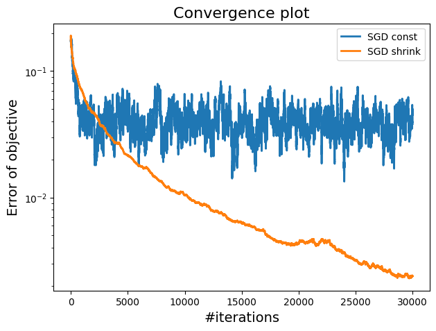
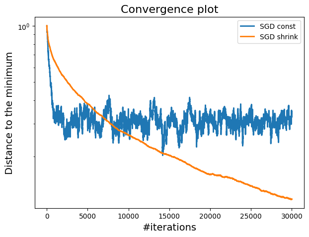
By comparing these two methods, we can see that while constant step sizes may be faster initially it tends to oscillate around the minimum as the iteration increases, shrinking step sizes provide a more reliable path to convergence, making them a preferred choice in scenarios where stability and accuracy are critical.
SGD with Switching to Shrinking Step Sizes
It’s often beneficial to start with a larger, constant step size for faster convergence early on, and then transition to smaller, shrinking step sizes to fine-tune the solution.
Constant Step Size (Early Iterations)
For the first \(t^*\) iterations, we use a constant step size: \begin{equation} \label{eq:const_to_switch} \gamma_t = \frac{1}{2L_{\max}} \end{equation} This ensures rapid progress toward minimizing the objective function.
Switching to Shrinking Step Sizes (Later Iterations)
After \(t^*\), we switch to a shrinking step size: \begin{equation} \gamma_t = \frac{2t + 1}{(t + 1)^2 \mu}, \end{equation} where, \(\mu\) is the strong convexity constant of the function, and the shrinking step size ensures that the updates become more conservative as the algorithm nears the optimal solution, which helps to reduce oscillations and improving stability.
Switch Point
The switch occurs at the iteration index \(t^*\), which is determined by the condition: \begin{equation} t^* = 4 \times \lceil \kappa \rceil, \end{equation} where \(\kappa = \frac{L_{\max}}{\mu}\) is the condition number of the problem. This point is chosen to balance between fast initial convergence and the need for more precision as we get closer to the solution.
Let’s now implement the above.
1
2
3
4
5
6
7
8
9
10
11
12
13
14
mu = model.mu_constant()
Kappa = Lmax/mu
tstar = 4 * int(np.ceil(Kappa))

steps_switch = np.zeros(n_iter + 1)
for i in range(n_iter):
    if i <= tstar:
        steps_switch[i] = 1 / (2 * Lmax)
    else:
        steps_switch[i] = (2 * i + 1) / ((i + 1) ** 2 * mu)

indices = np.random.choice(n, n_iter + 1, replace=True)
np.size(indices)
w_sgdss, obj_sgdss, err_sgdss = sgd(w0, model, indices, steps_switch, w_min, n_iter)
This switching approach effectively combines the advantages of both constant and shrinking step sizes as the constant step size in the early iterations allows for quick progress toward reducing the objective function and as we approach the minimum, the gradients become smaller, and the shrinking step sizes help to ensure that the updates do not overshoot the minimum.
Comparing SGD with Constant to Switching Step Sizes
Let’s now compare the difference between SGD with constant step size and shrinking step size and observe their rate of convergence.
1
2
3
4
5
6
7
8
9
10
11
12
13
14
15
16
17
18
19
20
# Plotting to compare with constant stepsize
plt.figure(figsize=(7, 5))
plt.semilogy(obj_sgdcr - obj_min, label="SGD const", lw=2)
plt.semilogy(obj_sgdss - obj_min, label="SGD switch", lw=2)
plt.title("Convergence plot", fontsize=16)
plt.xlabel("#iterations", fontsize=14)
plt.ylabel("Error of objective", fontsize=14)
plt.legend()
plt.axvline(x=tstar, color = "orange", linestyle='dashed')

# Distance to the minimizer on a logarithmic scale
plt.figure(figsize=(7, 5))
plt.yscale("log")
plt.semilogy(err_sgdcr, label="SGD const", lw=2)
plt.semilogy(err_sgdss , label="SGD switch", lw=2)
plt.title("Convergence plot", fontsize=16)
plt.xlabel("#iterations", fontsize=14)
plt.ylabel("Distance to the minimum", fontsize=14)
plt.legend()
plt.axvline(x=tstar,  color = "orange", linestyle='dashed')
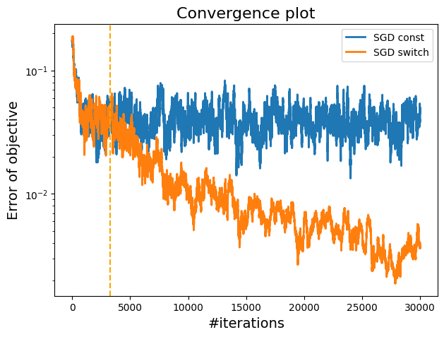
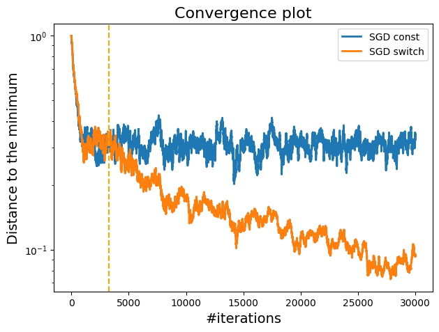
The plot demonstrates that the switch to shrinking stepsizes strategy outperforms the constant stepsize approach by reducing the oscillations and providing a smoother convergence towards the minimum.
SGD With Averaging
One powerful technique that can enhance the performance of SGD is averaging. Averaging works by calculating the mean of the iterates towards the end of the optimization process
Here, start averaging the iterates only in the last quarter of the total iterations. This allows the algorithm to have more information to average on. Let’s implement it.
1
2
3
4
5
6
# Implementing averaging with SGD
indices = np.random.choice(n, n_iter+1, replace=True)
start_late_averaging = 3*n_iter/4
averaging_on = True

w_sgdar, obj_sgdar, err_sgdar = sgd(w0, model, indices, steps_switch, w_min, n_iter, averaging_on, 0.0, True, start_late_averaging)
Comparing the Results.
Let’s now compare the difference between SGD with constant, switching and averaging step size and observe their rate of convergence.
1
2
3
4
5
6
7
8
9
10
11
12
13
14
15
16
17
18
19
20
21
22
23
# Plotting to compare constant stepsize, switchting, switching + averaging
plt.figure(figsize=(7, 5))
plt.semilogy(obj_sgdcr - obj_min, label="SGD const", lw=2)
plt.semilogy(obj_sgdss - obj_min, label="SGD switch", lw=2)
plt.semilogy(obj_sgdar - obj_min, label="SGD average end", lw=2)
plt.title("Convergence plot", fontsize=16)
plt.xlabel("#iterations", fontsize=14)
plt.ylabel("Loss function", fontsize=14)
plt.legend()
plt.axvline(x=tstar, color = "orange", linestyle='dashed')
plt.axvline(x=start_late_averaging, color = "green", linestyle='dashed')

# Distance to the minimizer on a logarithmic scale
plt.figure(figsize=(7, 5))
plt.semilogy(err_sgdcr, label="SGD const", lw=2)
plt.semilogy(err_sgdss , label="SGD switch", lw=2)
plt.semilogy(err_sgdar , label="SGD average end", lw=2)
plt.title("Convergence plot", fontsize=16)
plt.xlabel("#iterations", fontsize=14)
plt.ylabel("Distance to the minimum", fontsize=14)
plt.legend()
plt.axvline(x=tstar, color = "orange", linestyle='dashed')
plt.axvline(x=start_late_averaging, color = "green", linestyle='dashed')

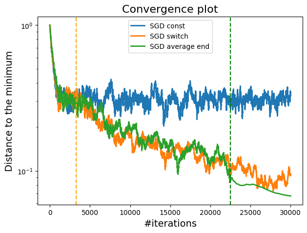
We can see that the averaging technique (green line) helps to stabilize the objective function, especially towards the end of the optimization process. This method is particularly useful when we want to ensure that the algorithm converges to a solution that generalizes well, as it mitigates the risk of overfitting due to fluctuations in the later stages.
SGD with Momentum
Momentum is a technique used to accelerate convergence, especially in scenarios where gradients oscillate. By adding a fraction of the previous update to the current update, this method potentially lead to faster convergence. Please note that I have already given and explained the updare rule for SGD with momentum in \(\eqref{eq:momentum}\).
Now let’s implement SGD with momentum:
1
2
3
4
5
indices = np.random.choice(n, n_iter+1, replace=True)
averaging_on = True
start_late_averaging = 0.0
momentum = 1.0
w_sgdm, obj_sgdm, err_sgdm = sgd(w0,model, indices, steps_switch, w_min, n_iter, averaging_on, momentum, True, start_late_averaging)
For simplicity, we have set the momentum parameter to \(1\). However, you can work with different values of momentum to check which one works best.
Comparing the Results
Let’s now compare the performance of SGD with constant step size, switching step size, switching step size with averaging, and SGD with momentum.
1
2
3
4
5
6
7
8
9
10
11
12
13
14
15
16
17
18
19
20
21
22
23
24
25
# Plotting to compare constant stepsize, switchting, switching + averaging
plt.figure(figsize=(7, 5))
plt.semilogy(obj_sgdcr - obj_min, label="SGD const", lw=2)
plt.semilogy(obj_sgdss - obj_min, label="SGD switch", lw=2)
plt.semilogy(obj_sgdar - obj_min, label="SGD average end", lw=2)
plt.semilogy(obj_sgdm - obj_min, label="SGDm", lw=2)
plt.title("Convergence plot", fontsize=16)
plt.xlabel("#iterations", fontsize=14)
plt.ylabel("Loss function", fontsize=14)
plt.legend()
plt.axvline(x=tstar, color = "orange", linestyle='dashed')
plt.axvline(x=start_late_averaging, color = "purple", linestyle='dashed')

# Distance to the minimizer on a logarithmic scale
plt.figure(figsize=(7, 5))
plt.semilogy(err_sgdcr, label="SGD const", lw=2)
plt.semilogy(err_sgdss , label="SGD switch", lw=2)
plt.semilogy(err_sgdar , label="SGD average end", lw=2)
plt.semilogy(err_sgdm , label="SGDm", lw=2)
plt.title("Convergence plot", fontsize=16)
plt.xlabel("#iterations", fontsize=14)
plt.ylabel("Distance to the minimum", fontsize=14)
plt.legend()
plt.axvline(x=tstar, color = "orange", linestyle='dashed')
plt.axvline(x=start_late_averaging, color = "purple", linestyle='dashed')
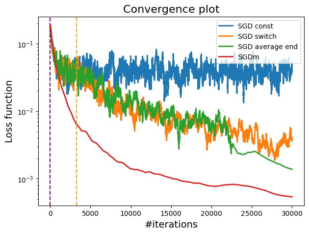
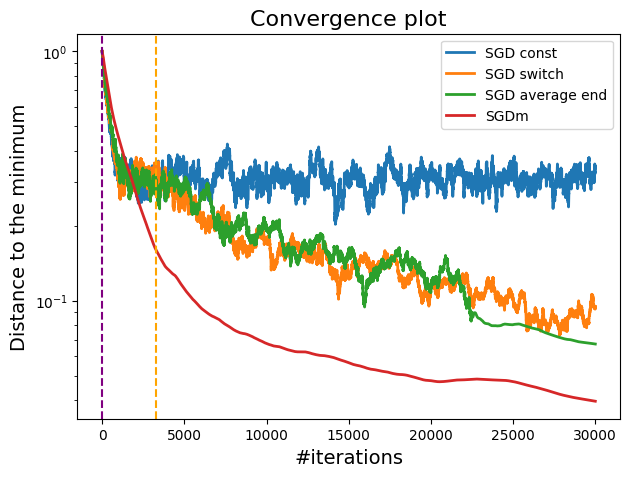
We can observe that SGD with momentum (red curve) shows the fastest convergence, outperforming other methods in both loss reduction and distance to the minimum. The vertical dashed lines indicate the point at which the step size switching occurs and where the late averaging begins.
SGD without Replacement
SGD without replacement selects each data point exactly once per epoch, ensuring that the model sees the entire dataset in each pass without replacement.
1
2
3
4
5
import numpy.matlib
niters = int(datapasses * n) - 1
indices = np.matlib.repmat(np.random.choice(n, n, replace = False), 1, datapasses)
indices = indices.flatten()
w_sgdsw, obj_sgdsw, err_sgdsw = sgd(w0, model, indices, steps_switch, w_min, niters)
Compare Result
Let’s now compare the performance of SGD with replacement and without replacement.
1
2
3
4
5
6
7
8
9
10
11
12
13
14
15
16
17
18
19
# Error of objective on a logarithmic scale
plt.figure(figsize=(7, 5))
plt.yscale("log")
plt.plot(obj_sgdss - obj_min, label="SGD with replacement", lw=2)
plt.plot(obj_sgdsw - obj_min, label="SGD without replacement", lw=2)
plt.title("Convergence plot", fontsize=16)
plt.xlabel("#iterations", fontsize=14)
plt.ylabel("Distance to the minimum", fontsize=14)
plt.legend()

# Distance to the minimizer on a logarithmic scale
plt.figure(figsize=(7, 5))
plt.yscale("log")
plt.plot(err_sgdss , label="SGD replacement", lw=2)
plt.plot(err_sgdsw , label="SGD without replacement", lw=2)
plt.title("Convergence plot", fontsize=16)
plt.xlabel("#iterations", fontsize=14)
plt.ylabel("Distance to the minimum", fontsize=14)
plt.legend()
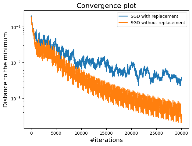
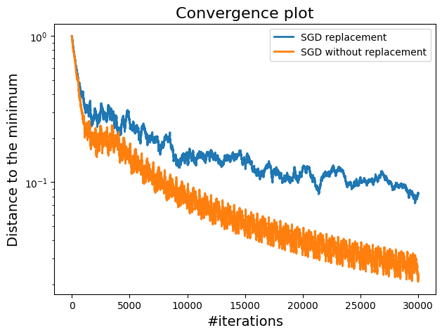
SGD without replacement demonstrates a better convergence to the minimum, likely due to the efficiency of utilizing the dataset without replacement. This method is generally more efficient because it avoids redundant updates and thus lead to faster convergence.
Comparing Gradient Descent with Stochastic Gradient Descent
After looking at various forms of Stochastic Gradient Descent (SGD), it’s important to compare these results with the traditional Gradient Descent (GD) method.
Gradient Descent Implementation
In each iteration of the gradient descent algorithm, the gradient is computed using the entire dataset, and the model’s weights are updated accordingly.
1
2
3
4
5
6
7
8
9
10
11
12
13
14
15
16
17
18
19
20
21
22
23
24
25
26
27
28
29
30
31
32
33
def gd(w0, model, step, w_min =[], n_iter=100, verbose=True):
    """Gradient descent algorithm
    """
    w = w0.copy()
    w_new = w0.copy()
    n_samples, n_features = X.shape
    # estimation error history
    errors = []
    err = 1.
    # objective history
    objectives = []
    # Current estimation error
    if np.any(w_min):
        err = norm(w - w_min) / norm(w_min)
        errors.append(err)
    # Current objective
    obj = model.f(w)
    objectives.append(obj)
    if verbose:
        print("Lauching GD solver...")
        print(' | '.join([name.center(8) for name in ["it", "obj", "err"]]))
    for k in range(n_iter ):
        w[:] = w - step * model.grad(w)
        obj = model.f(w)
        if (sum(w_min)):
            err = norm(w - w_min) / norm(w_min)
            errors.append(err)
        objectives.append(obj)
        if verbose:
            print(' | '.join([("%d" % k).rjust(8),
                              ("%.2e" % obj).rjust(8),
                              ("%.2e" % err).rjust(8)]))
    return w, np.array(objectives), np.array(errors)
To ensure stable convergence in Gradient Descent, we select the step size (step) as the inverse of the Lipschitz constant of the gradient:
1
2
3
step = 1. / model.lipschitz_constant()
w_gd, obj_gd, err_gd = gd(w0, model, step, w_min, datapasses)
print(obj_gd)
To fairly compare GD with SGD, we calculate the computational complexity of GD. Since each step of GD requires a full pass over the dataset, the total computational effort can be represented as:
1
complexityofGD = n * np.arange(0, datapasses + 1)
Compare Results
Let’s now compare the performance of SGD with GD.
1
2
3
4
5
6
7
8
9
10
11
12
13
14
15
16
17
18
19
# Error of objective on a logarithmic scale
plt.figure(figsize=(7, 5))
plt.semilogy(complexityofGD, obj_gd - obj_min, label="gd", lw=2)
plt.semilogy(obj_sgdss - obj_min, label="sgd switch", lw=2)
plt.semilogy(obj_sgdm - obj_min, label="sgdm", lw=2)
plt.title("Convergence plot", fontsize=16)
plt.xlabel("# SGD iterations", fontsize=14)
plt.ylabel("Loss function", fontsize=14)
plt.legend()

# Distance to the minimum on a logarithmic scale
plt.figure(figsize=(7, 5))
plt.semilogy(complexityofGD, err_gd, label="gd", lw=2)
plt.semilogy(err_sgdss , label="sgd switch", lw=2)
plt.semilogy(err_sgdm , label="sgd switch", lw=2)
plt.title("Convergence plot", fontsize=16)
plt.xlabel("# SGD iterations", fontsize=14)
plt.ylabel("Distance to the minimum", fontsize=14)
plt.legend()
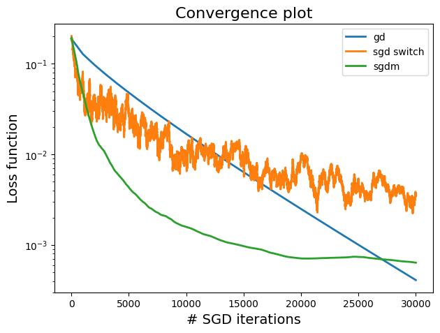
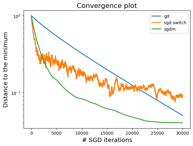
From our comparison, SGD variants are more computationally efficient compared to GD. They make faster progress in the initial stages, which is crucial in large-scale datasets. GD provides more stable convergence but at a higher computational cost.
Comparing Test Error: Gradient Descent vs. SGD with Momentum
In this final comparison, we focus on the test error, which is important for understanding how well our models generalize to unseen data.
1
2
3
4
5
6
7
8
9
10
11
12
13
14
15
16
17
18
19
20
21
22
23
24
25
26
datapasses = 30;
n_iters = int(datapasses * n)
# With replacement
indices = np.matlib.repmat(np.random.choice(n, n, replace = False), 1, datapasses)
indices = indices.flatten()
##
steps = 0.25 / np.sqrt(np.arange(1, niters + 2))

indices = np.random.choice(n, n_iter+1, replace=True)
w_sgdar, obj_sgdar, err_sgdart    = sgd(w0,model, indices, steps_switch, w_model_truth, n_iter, True, False, 3*n_iter/4) # (datapasses-5)*n

w_sgdsw, obj_sgdsw, err_sgdswt = sgd(w0,model, indices, steps, w_model_truth, n_iter, verbose = False);
## GD
step = 1. / model.lipschitz_constant()
w_gd, obj_gd, err_gd = gd(w0, model, step, w_model_truth, datapasses, verbose = False)
complexityofGD = n * np.arange(0, datapasses + 1)

## SGD with momentum
averaging_on = True
start_late_averaging = 0.0
momentum = 1.0
w_sgdm, obj_sgdm, err_sgdmt = sgd(w0,model, indices, steps_switch, w_model_truth, n_iter, averaging_on, momentum, True, start_late_averaging) # (datapasses-5)*n

## GD
step = 1. / model.lipschitz_constant()
w_gd, obj_gd, err_gdt = gd(w0, model, step, w_model_truth, datapasses)
Compare Result
Let’s compares the test error convergence for Gradient Descent (GD) and Stochastic Gradient Descent with Momentum (SGDm).
1
2
3
4
5
6
7
8
9
10
11
# Distance to the minimizer on a logarithmic scale
plt.figure(figsize=(7, 5))
plt.yscale("log")
plt.semilogy(complexityofGD, err_gdt , label="GD", lw=2)
# plt.semilogy(err_sgdswt, label="SGD without replacement", lw=2)
# plt.semilogy(err_sgdart , label="SGD averaging end", lw=2)
plt.semilogy(err_sgdmt,  label="SGDm", lw=2)
plt.title("Convergence plot", fontsize=16)
plt.xlabel("#iterations", fontsize=14)
plt.ylabel("Test error", fontsize=14)
plt.legend()
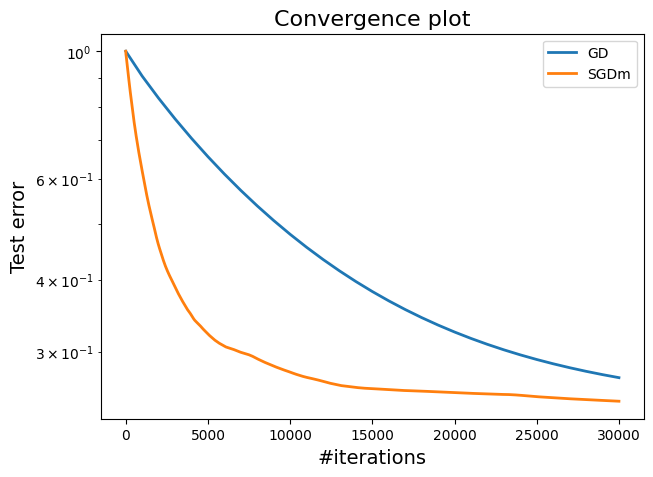
From the plot, SGDm not only converges faster but also achieves a lower final test error compared to GD. This indicates better generalization, making SGDm more suitable for real-world applications where test performance is critical.
Conclusion
By comparing these methods with Gradient Descent, we’ve highlighted the practical advantages of SGD, particularly in handling large-scale datasets where computational efficiency is key. Our final comparison of test error revealed that SGD with momentum not only accelerates convergence but also leads to superior model performance, making it a powerful method.